Roofline Analysis of Dot Product on an H100

13 Feb, 2025

Summary

Algorithms spend time in two places:

Computation, where the time is spent performing arithmetic operations such as multiplying and adding floating point numbers. For example, a H100 GPU can perform 989 TFLOPs of TF32 operations per second.
Communication, where the time is spent moving data within the GPU (b/w the cores and the HBM) or across the GPUs. The HBM bandwidth of a H100 is 3.35 TB/s and for GPU-to-GPU communication using Nvidia NVLink it is 900 GB/s.

Let $T_{m a t h}$ be the time spent in computation and $T_{c o m m s}$ be the time spent in communication.

$T_{m a t h} = \frac{Computation FLOPs}{Accelerator FLOPs/s}$

$T_{c o m m s} = \frac{Communication GB}{Network/Memory Bandwidth GB/s}$

We can lowerbound the time take by an algorithm by assuming we can perfectly overlap communication with computation. $$ T_{lowerbound} = \max(T_{math}, T_{comms}) $$

And we can upperbound the time taken by assuming zero overlap.

T_{u p p e r b o u n d} = T_{m a t h} + T_{c o m m s}

We will optimize the algorithm to with respect to the $T_{l o w e r b o u n d}$ i.e., maximizing the overlap between computation and communication.

Assuming we can perfectly overlap communication with computation, we will have one of the following two cases:

$T_{c o m m s} > T_{m a t h}$ : Algorithm is memory or communication bound. Some fraction of the accelerator FLOPs/s are spent waiting for data movement.
$T_{m a t h} > T_{c o m m s}$ : Algorithm is compute bound. All the accelerator FLOPs/s are being used to compute i.e., we see full utilization of the compute capability of the hardware.

A proxy measure for checking if an algorithm is compute bound is the arithmetic intensity of the algorithm which measures FLOPs per byte of data moved. It is the ratio of the FLOPs the algorithm performs to the number of bytes it needs to move.

Arithmetic Intensity = \frac{Computation FLOPs}{Communication Bytes}

We can derive the following simple theorem relating the arithmetic intensity of an algorithm and intensity of the accelerator that can help us figure out if an algorithm is compute bound or not:

$T_{m a t h} > T_{c o m m s}$

$⟺ \frac{Computation FLOPs}{Accelerator FLOPs/s} > \frac{Communication GB}{Network/Memory Bandwidth GB/s}$

$⟺ \frac{Computation FLOPs}{Communication GB} > \frac{Accelerator FLOPs/s}{Network/Memory Bandwidth GB/s}$

$⟺ Arithmetic Intensity > \frac{Accelerator FLOPs/s}{Network/Memory Bandwidth GB/s}$

$⟺ Arithmetic Intensity & > Accelerator Intensity$

Arithmetic Intensity of Dot Product

The dot product of two vectors is a fundamental operation in many algorithms, including neural networks. Let’s analyze the arithmetic intensity of the dot product operation and see if it’s compute bound or not on an H100 GPU.

The dot product of two vectors $𝐚$ and $𝐛$ of size $N$ is defined as:

𝐚 \cdot 𝐛 = \sum_{i = 1}^{N} a_{i} \cdot b_{i}

Let’s find the arithmetic intensity of the dot product operation on vectors in bfloat16 precision. Each vector has $N$ elements requiring $2 N$ bytes of memory. So, together the two vectors require $4 N$ bytes of memory and writing the result back requires 2 bytes. Dot product requires $N$ multiplications and $N - 1$ additions which makes the total number of operations $2 N - 1$ .

Arithmetic Intensity = \frac{Computation FLOPs}{Communication Bytes} = \frac{2 N - 1}{4 N + 2}

As $N$ approaches infinity, the arithmetic intensity approaches $\frac{1}{2}$ . In other words, the dot product operation does 0.5 FLOPs per byte of data moved. Let’s compare this with the peak arithmetic intensity of the H100 SXM GPU.

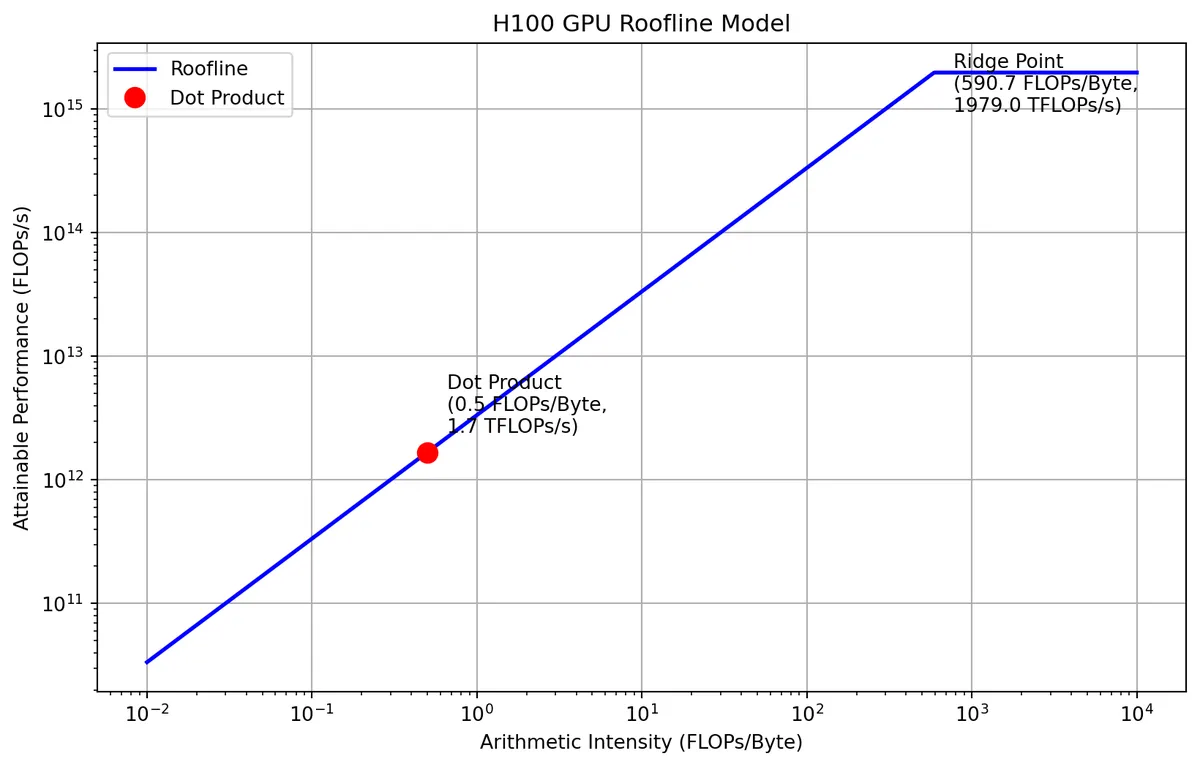
H100 Peak Arithmetic Intensity = \frac{1979 * 10^{12} FLOPs/s}{3.35 * 10^{12} Bytes/s} = 590.7 FLOPs/Byte

The arithmetic intensity of the dot product is way less than the peak arithmetic intensity of the H100. This means that the dot product operation is memory bound and its performance can be improved by either increasing the bandwidth of the memory or by increasing the arithmetic intensity of the algorithm.

To make this clear, let’s plot a roofline for the dot product operation on an H100 GPU. The y-axis is the peak intensity of the H100 (FLOPs/s) and the x-axis is the arithmetic intensity of our algorithm.

Roofline plot for the dot product operation on an H100
GPU

Code

import numpy as np
import matplotlib.pyplot as plt

# H100 specs
H100_PEAK_FLOPS = 1979e12  # FLOPs/s
H100_MEMORY_BW = 3.35e12   # Bytes/s
H100_PEAK_INTENSITY = H100_PEAK_FLOPS / H100_MEMORY_BW

# Generate x-axis points for arithmetic intensity
x = np.logspace(-2, 4, 1000)  # Log scale from 0.01 to 10000

# Calculate attainable performance
memory_bound = H100_MEMORY_BW * x  # Diagonal line
compute_bound = np.full_like(x, H100_PEAK_FLOPS)  # Horizontal line
attainable_perf = np.minimum(memory_bound, compute_bound)

# Dot product arithmetic intensity and its achievable performance
dot_product_intensity = 0.5  # FLOPs/Byte
dot_product_performance = H100_MEMORY_BW * dot_product_intensity  # Memory-bound performance

# Ridge point (point of inflection)
ridge_point_x = H100_PEAK_INTENSITY
ridge_point_y = H100_PEAK_FLOPS

# Plot in log-log scale
plt.figure(figsize=(9, 6))
plt.loglog(x, attainable_perf, 'b-', linewidth=2, label='Roofline')
plt.plot(dot_product_intensity, dot_product_performance, 'ro', markersize=10, label='Dot Product')

# Add annotations
plt.annotate(f'Dot Product\n({dot_product_intensity:.1f} FLOPs/Byte,\n{dot_product_performance/1e12:.1f} TFLOPs/s)',
            (dot_product_intensity, dot_product_performance),
            xytext=(10, 10), textcoords='offset points')

plt.annotate(f'Ridge Point\n({ridge_point_x:.1f} FLOPs/Byte,\n{ridge_point_y/1e12:.1f} TFLOPs/s)',
            (ridge_point_x, ridge_point_y),
            xytext=(10, -20), textcoords='offset points')

plt.grid(True)
plt.xlabel('Arithmetic Intensity (FLOPs/Byte)')
plt.ylabel('Attainable Performance (FLOPs/s)')
plt.title('H100 GPU Roofline Model')
plt.legend()
plt.show()

#AI #GPUs #engineering